ECE 209 Notes

Table of Contents

1. Materials Structure
2. Atomic Structure
3. Band Structure
4. Metals
5. Optics
6. Dielectrics
7. Thermal Properties
8. Magnetic Properties

Materials Structures

Crystalline, polycrystalline, and amorphous

• materials can be classified into the 3 types: crystalline, polycrystalline, and amorphous

Crystalline

• crystalline solid: a solid in which atoms bond in a regular pattern to form a periodic array of atoms
• long range order: happens in a crystalline solid b/c periodicity;
  • means that each atom is in the same position relative to its relative
  • perfect order yay

Polycrystalline

• long-range order exists over small distances only
• has small crystal “grains” that are randomly oriented

Amorphous

• no long-range order! It’s completely disordered

Crystals in microelectronics

• different types of crystals should be used for different things in microelectronics
• Polycrystalline silicon used for:
  • gate material in MOS transistors
  • interconnect lines
• Amorphous silicon used for:
  • switching transistors for AMLCD displays
  • solar cells
• crystalline used for all kinds of things
  • attractive because of perfect order, which:
    • simplifies theories
    • repeatable, predictable and uniform properties for material processing

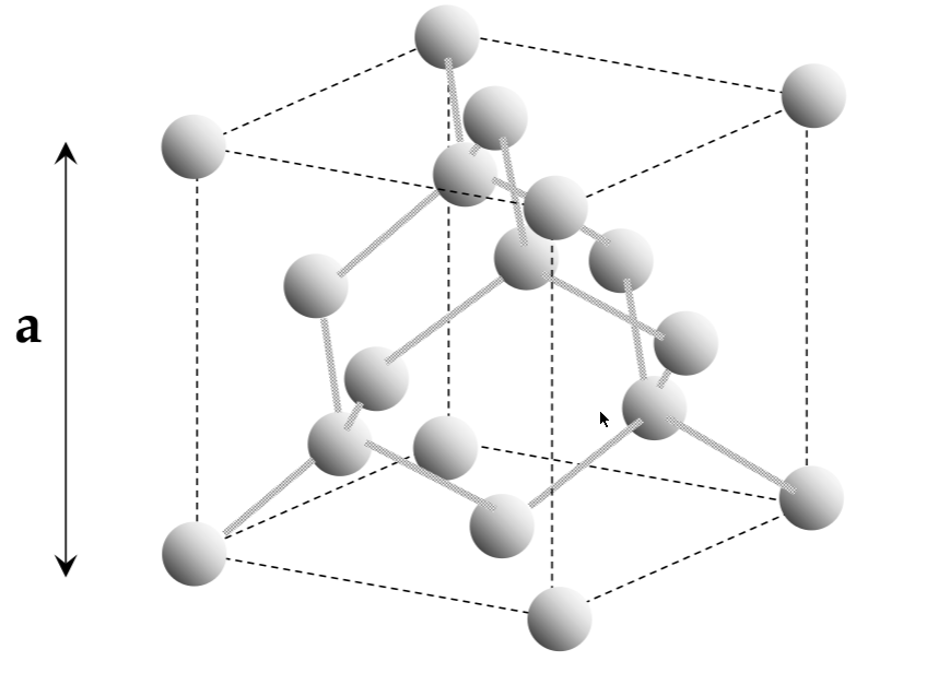
Silicon structure; covalent bonding

• covalent bonding: shares atoms to make a full valence shell (8 atoms for Si)
  • Si ends up in a tetrahedral shape due to the repulsion interactions
• silicon has a diamond unit cell

Unit cell

• lattice: infinitely repeating array of geometric points in space
• lattice crystal structure: a lattice, with atoms on the lattice points
• unit cell: smallest repeating structure in the lattice crystal structure
  • lattice constant: the length of the cubic unit cell - a
  • interatomic distance: the distance between atoms in a unit cell (not the same as a!!)

Bragg’s Law

• to measure the lattice constant of an atom, use x-ray diffraction
• for a wave incident on a plane of atoms, reflective pattern will have bright and dark spots from constructive and destructive interference
• Bragg’s Law for where bright spots appear:
  $$ n\lambda = 2dsin\theta $$

- crystal characteristics (and x-ray diffraction) depend on the direction you are looking

Miller indices

• since direction matters, we need a way of classifying it
• miller indices: sets of 3 numbers that are used to identify groups of crystal planes and directions

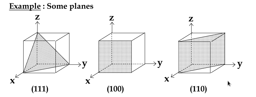
Miller Indices for Planes

• set up 3 axes along 3 adjacent edges of unit cell
• choose unit cell length as unit distance along respective axis (a = 1)
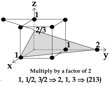
• chose a plane that passes through the centre of particular atoms. The plan intersects the axes at distances x1,y1, za (in example below, 1,2, 2/3)
• take reciprocals of interception co-ordinates, change to set of smallest ints, write as (hkl)

Miller Indices for Directions

• take a parallel line which passes through the origin
• not the length of the projections of this line on x,y,z axes
• change to smallest ints
• write as [hkl]

Family of Planes and Directions

• family of planes: {hkl)
• family of directions:
• represents all equivalent planes/directions
• {110} represents all planes (110), (011), (101), etc

Transmission Electron Microscopy

• TEM samples thinned and illuminated with accelerated electrons
• electrons are absorbed in the sample depending on thickness and material composition
• intensity variation of the transmitted electron beam is observed using a viewing screen

Scanning Tunneling Microscopy

• scans across the surface of sample with a very sharp needle
• needle kept 1nm from surface, voltage applied between needle and sample
• current used as feedback signal to determine gap size (can only give information about surface of sample)

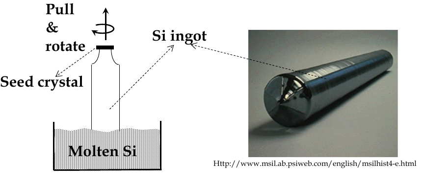
Silicon bulk crystal growth

• to make ICs, we have to grow perfect crystals on a commercial scale
• for crystal growth, a saturated solution or a molten liquid is usually used.
• the material is then grown on a seed crystal which acts as a template for the new growth
• for silicon:
  • raw material: silicon dioxide
  • reduction => metallurgical grade polycrystalline Si
  • purification => electronic grade polycrystalline Si
  • melting & growth => crystalline bulk Si
• during melting and growth, a seed crystal is pulled slowly out of a bath of molten and rotated slowly
  • this is Czochralski (Cz) crystal pulling
• after growth, ingot is trimmed and sliced into wafers

Epitaxial growth

• electrical properties of Si are controlled roughly when the basic wafers are produced, but more precise cotrol is needed for reliable devices
• the top few microns of the wafer are where devices are made
  • this region must be well controlled
• achieved by growing a even more perfect crystal layer on top of the wafer
  • called the epitaxial layer
• during epitaxial growth, the surface of the wafer acts as the template
• decomposes Si-containing gases in chemical vapor dposition
• monolayer : a layer one atom thick

Molecular beam epitaxy

• a technique for growing thin layers
• a steam of neutral atoms or molecules are evaporated from a heated cell
• then incorporated into the growing film onto a heated target
• is $$$ $ b/c:
  • only one wafer can be used at a time
  • wafer must be small to get uniform layer
  • very good vacuum required

Epitaxy principles

• major feature of epitaxy is that the newly deposited film precisely follows the crystalline form of the substrate template
• adsorption: proces of atoms attaching themselves to the surface
• adsorption can occur anywhere on the surface with equal probability, so layer is unlikely to be crystalline
• for crystalline growth, absorbed atoms must be able to find the minimum energy positions
  • the ad-atoms must be able to move along the surface
• heat up the substrate during epitaxy to allow movement
  • if not hot enough, the ad-atoms stick where they land and the film is amorphous

Modifying Crystals

• to make an electronic device, crystals need to be modified and shaped according to the needs of the device
• examples: introducing impurities, etching/shaping

Ion implantation

• ionized impurities are accelerated into an electric field and “smashed into” Si surface
• depth of penetration determined by:
  • accelerating voltage
  • masses of ions and target atoms
  • crystal direction (density of atoms)

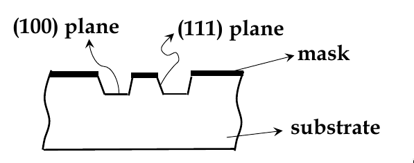
Etching and micromachining

• sometimes you need to etch crystals to get certain structures
  e.g. for making DRAMs, you need to etch deep tranches to make trench-capacitors
• wet-etching: uses liquid chemicals to remove materials from a wafer
• isotropic etching: chemicals etch at the same rate in all directions
• anisotropic etching: chemicals selectively etch one crystal plane more
  • see example below. KOH etches (100) faster than (111) planes

Atomic Structure

Nature of light

• classic physics: light is an electromagnetic wave w/ perpendicular field Bx and Ey
• electric field is given by the following equation:
  $$ E_y = E_o sin(kx - \omega t) $$
• where:
  • k = 2π/λ - the wavenumber (λ is the wavelength of light)
  • ω = 2πf - the angular frequency (f is the freq of light)
  • c= ω/k = fλ - speed of light / wave velocity
• light intensity is given by:
  $$ I = \frac{1}{2} c \epsilon_o E_o^2 $$

Experimental Evidence of Light as EM Wave

• interference and diffraction
• Young’s double-slit experiment
  • expand

Photo-emission (photoelectric effect)

• when a metal electrode is illuminated with light, it emits electron (can create a current with this!)
• light must possess the energy needed to “free” the electron from the metal (W)
  • any excess energy it possesses will become the kinetic energy of the electron
• according to classical theory of light, the energy balance should be: E _L = W + E _K
  • if we reduce E _L by reducing the intensity of the light, E _K should also decrease
• if light intensity is increased -> saturation current increases
  • more electrons emiited
  • same voltage is required to stop the current, thus the kinetic energy of the electrons is the same
• classical theory of light can’t explain this!

Photons

• light contains particle of fixed energy called photons
• light frequency increases -> energy of light increases
• E _L = hf
  • h = Planck’s constant

Wave-Particle Duality

• light has properties of both a wave and a particle
• light waves consist of a stream of photon particles, each with energy hf
  • energy carried by the wave consists of discrete lumps or quanta

De Broglie relationship

• electrons also have a wave-particle duality
• particle-like properties confirm with cathode ray tube (1897)
• deBroglie predicted that electrons would have a wavelength:
  $$ \lambda = \frac{h}{p} $$
  • where p = mv is the electron momentum
• confirmed with electron diffraction experiment

Electron Diffraction Experiment

• voltage accelerates electron, strikes a thin carbon layer, hits the screen
  • produce a glow of light proportional to their number and energy
    
• using this, get the deBroglie relationship

Wavefunction, wave vector, and Schrödinger equation

• for an electromagnetic wave:
  $$ E_y (x,t) = E_o sin(kx - \omega t) $$
• for an electron wave:
  $$ \psi = A sin(kx - \omega t) $$
  $$ \psi = Ae^{j(kx - \omega t)} $$
• where:
  • k = 2π/λ - the wave vector
  • ω = 2πf
  • A = constant
• can separate the time-dependent and space-dependent parts and write:
  $$ \psi = Ae^{jkx}e^{-j\omega t}$$
• wave function related to the probability of finding the electron at a given point in space and time
  • represents the distribution of the electron wave in time
• Probability = ΨΨ* = |Ψ| ²
  • probability is a real value

Wave Vector and Potential Energy

• electron wave momentum is related to the wavelength by this equation: p = h/v
• momentum is a vector - therefore we need a vector form of the wavelength
• wave vector:
  • direction: direction of wave travel
  • magnitude: k = 2π\λ
• momentum now written as:
  $$ p = \frac{h}{2π}k$$
• kinetic energy is:
  $$ E_k = \frac{p^2}{2m} = \frac{h^2}{8π^2}\frac{k^2}{m}$$
• electron also has electrostatic potential energy
  • defined as the work done in pulling the negatively chargely electron from an infinite distance to a distance, r, from the positively charged nucleus:
    $$ E_p = \frac{-e^2}{4πε_0 r} $$
    -total energy is E = E _k + E _p
    $$ k = \frac{2π}{h} \sqrt{2m(E - E_p)} $$

Schrodinger’s Equation

• describes the electron wave function
• if you know the electron potential energy and boundary conditions, you can calculate the parameters of electron orbital (wave function and energy)
  $$ \frac{d^2 \Psi}{dx^2} + \frac{8\pi^2 m}{h^2}(E - E_p )\Psi = 0 $$

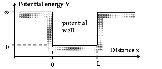
“Electron in a box” problem

Electron in a 1D Potential Well

-setup:
- inside the box, potential energy is zero
- outside, is infinitely large
- we need to find the wave equation

$$ \frac{d^2 \Psi}{dx^2} + \frac{8\pi^2 m}{h^2}(E - V)\Psi = 0 $$

• assumptions:

  • the case is time-independent
  • wave function is continuous, smooth, and single-

• Boundary conditions:

  1. For x<0 and x>L, the term Vψ dominates
     $$ -V\Psi = 0 \\ \Psi = 0 |\Psi|^2 = 0 $$
     electron cannot be outside the well
  2. Since d ² ψ/dx ² must be continuous, ψ = 0 at x={0,L}

• Differential equation:

  • second order differential equation to solve for within the well
  • general solution equation is:
    $$ \Psi (x) = 2Ajsin(\frac{n\pi x}{L}) $$
  • can solve for A because we know the probability of electron being in the box is 1 (integral of equation from 0 to L is 1)
  • final form of the equation is:
    $$ \Psi (x) = j(\frac{2}{L})^{\frac{1}{2}}sin(\frac{n\pi x}{L}) $$

Electron Energy in Potential Well

$$ E = \frac{h^2 n^2}{8mL^2} $$
- energies E(n) are the eigenenergies of the electron
- energy is quantized
- n is the quantum number
- min energy is at n=1, this is the ground state
- energy of electron wave can only have discrete values
- energy of electron particle can take any value

Uncertainty Principle

• free electron:
  • has single energy, momentum, wavelength - Δp = 0 (uncertainty 0)
  • electron wave is spread all over the space, so Δx = ∞
• electron in a potential well:
  • Δx = L
  • Δp = hk/π
    • for n=1, k: = π, Δp = h/L
      $$ \Delta x \Delta p = L \frac{h}{L} = h $$
• Heinsenberg’s uncertainty principle: we cannot simultaneously and exactly know both the position and momentum of an electron along a given co-ordinate

Tunnelling

• important application of the uncertainty principle
• if an electron of energy E meets a potential energy barrier of height V_o_ > E, it might leak (“tunnel”) throug the barrier
  • probability of that depends on the energy and width of the barrier

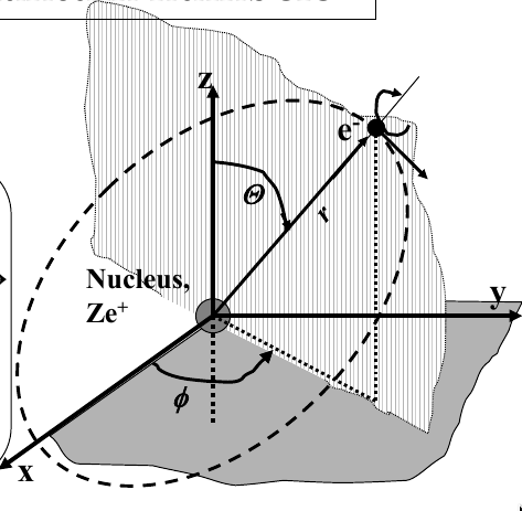
Hydrogen atom

• consider the H atom: an electron attached to a nucleus
  • electron is electrostatically bound to a single proton
  • since proton is so big, it behaves more like a particle
• potential energy:
  $$ V(r) = \frac{-Ze^2}{4\pi \epsilon_o r} $$
• where:
  • Z = number of electrons
  • r = (x ² + y ² 2 + z ² ) ^1/2
• considerng electron in H atom as confined in a potential well with PE V(r), electron’s wave function can be derived to be:
  $$ E = \frac{-Z^2 e^4 m}{8h^2 \epsilon_o^2}\frac{1}{n^2} $$
  • different energy values (different values on) are called Energy Levels

Atomic Spectra

• electrons can be excited into higher energy levels - requires energy
• they can also return to a lower levels - releases energy in the form of a photon with appropriate energy E = hf = E _higher - E _lower

Quantum Numbers

Principal Quantum Number, n

• determines the radius of electron orbit and the energy level

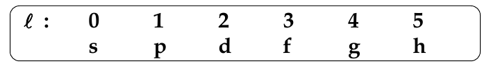
Orbital Angular Quantum Number, l

• determines the shape of the orbital
• the electron wave at each orbit (at each r) may be standing or moving along the orbit
• wave must be continuous and smoothly varying
  • must fit an integral number of wavelengths: lλ = 2πr
    $$ L = pr = \ell \frac{h}{2\pi} $$
• L is the angular momentum, which is quantized.
• l can take any value from 0 to (n-1)

Magnetic Quantum Number, m _l

• determines orientation of the orbital in space (the tilt of the electron cloud), and the energy of its electron in a magnetic field
• angular momentum about the electron orbit is quantized as:
  $$ L_z = \frac{m_\ell h}{2\pi} $$
• -l ≤ m _l ≤ l

Electron Spin Quantum Number, m _s

• determines the rotation of electron about its own axis
• has the values 1/2, -1/2 (spin up, spin down)

The Full Sert of Quantum Numbers and Values

n = 1, 2, 3, … z
l = 0, 1, 2, 3, … (z-1)
m _l = 0, ±1, ±2, ±3, … ±(z-1)
m _s = ±1/2

Summary of Quantum Numbers

• Radius of orbit → n
• Orbital angular momentum → l
• Tilt of orbit’s plane → m _l
• Spin of electron → m _s

Electron Clouds

• we can define electron clouds corresponding to different combos of quantum numbers
  • probability density distribution

Multi-electron atoms, Pauli principle, and the periodic table

• building atoms requires an organization of Z electrons around the nucleus
• two principles for doing so:
  • electrons will occupy the lowest possible available energy state
  • no more than one electron can have the same set of quantum numbers (Pauli’s Exclusion Principle)

• start filling the atomic states (quantum number states) with electrons

  • e.g.: For Lithium, there are 3 electrons:
    • n = 1, l = 0, m _l = 0, m _s = 1/2
    • n = 1, l = 0, m _l = 0, m _s = -1/2
    • n = 2, l = 0, m _l = 0, m _s = 1/2

• notation:
  
  

Band Structure

Hydrogen molecule and molecular bonding

• when atoms interact, they change behaviour
  • no two electrons in an interacting systems may occupy same quantum state
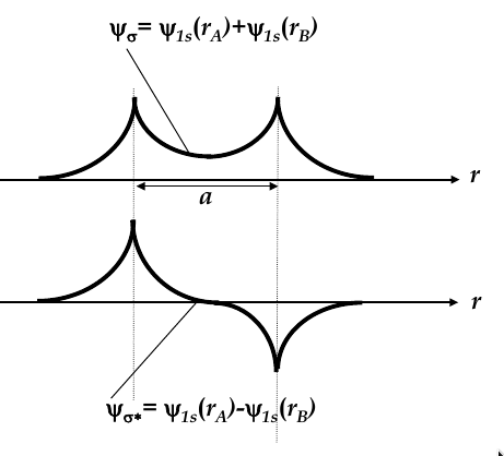
• consider the case of two H atoms
  • when they are infinitely far apart, they have the same wave function
  • when they approach each other, their wave functions overlap and two new molecular wave functions emerge (see the image below for the two new functions
• molecular wave functions are linear combinations of atomic orbitals; in this case, one is the sum and one is the difference
• Ψ _σ is more confined to the nuclei, whereas Ψ _σ* is more spread
  • thus, Ψ _σ* has higher energy
  • Ψ _σ then is more energetically favourable, so both electrons occupy this state
• bonding orbital: the wave function Ψ _σ corresponding to the lowest energy level
• antibonding orbital: Ψ _σ*
• total energy of two electrons in H ₂ molecule is lower than in two single H atoms
  • one electron has to flip its electron spin but the energy gain due to dropping to bonding orbital is higher than the energy spent

Energy band formation; metals, semiconductors and insulators

• consider 3 hydrogen atoms. They will also add their atomic wave functions, like so:
  
• the more atoms in our function, the more molecular orbitals they’ll form. n atoms = n orbitals
• if an energy band is not entirely filled, there are states available for electrons. Consider N Li atoms (2s half filled)
  • thermal energy is enough at room temp for electrons to jump between nearest energy levels
  • since the levels may belong to different atoms, electrons can easily travel from atom to atom conducting current

Hybridization

• 2s and 2p energy levels are close, so when they approach each other, 2 2s and 2 2p orbitals can mix to form hybrid orbitals
  • hybrid orbitals directed in tetrahedral directions and have the same energy
• process called sp ³ hybridization

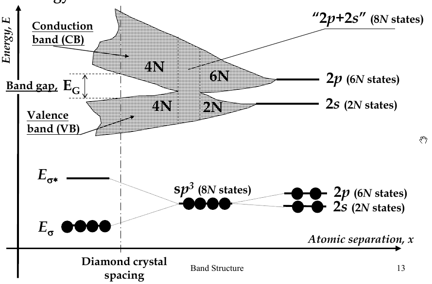
Energy Bands

• when interatomic distance decreases so that electrons interact, their energy levels broadens (splits) into bands
• there are 2N states in the 2s-band, 6N states in 2p-band
• in diamond crystal, bonding and anti-bonding orbitals split and form valence band and conduction band , respectively
• band gap - E _G - the difference in energy between the conduction and valence bands

Fermi Energy

• at T=0K, all electrons will occupy states with lowest energy (valence band), so conduction band empty
• fermi energy (E _F ) = energy level corresponding to highest filled electron state at 0K.
• as T increases, bands above E _F start to get filled
• to conduct electric current, there must be vacant states in the band
• no states available in energy levels within each band, no conduction

need more but confusing tho

Effective mass

• acceleration of an free electron in vacuum is a = F _ext / m _e , m _e = electron mass in vacuum
• in a solid, electron interacts with crystal lattice atoms and experiences internal forces F _int
• thus, acceleration is: a = (F _ext + F _int ) / m _e

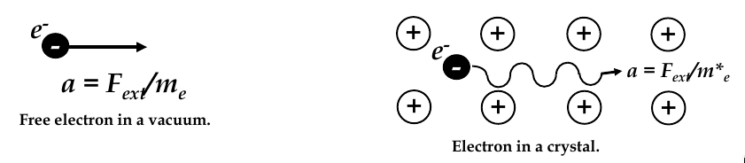
• since atoms in a crystalline solid are periodically positioned, variation of F _int is also periodic, we can simplify our acceleration equation:
  $$ a_crystal = \frac{F_ext}{m_e^*}
• where m _e ² is the effective mass of the electron
• effective mass depends on the material

Electrons and holes

• in semi-conductors, in order to get excited to empty states, electrons jump across the band gap
• when excited to the conduction band, a vacant state is left in the valence band
  • this is called a hole - the absence of an electron
• electrical conduction in a semiconductor involves movement of electrons in the conduction band and holes in valence band
  • electron and hole currents

Intrinsic Semiconductor

• a pure semiconductor (no foreign atoms present) is an intrinsic semiconductor
• electrons and holes can only be created in pairs (electron-hole pairs)

Carrier Generation

• electron-hole pair generation: the act of exciting an electron from the valence band to the conduction band
• electrons can be excited even though E _T is much smaller than E _G because atoms in the crystal are constantly vibrating (due to thermal energy) and deforming interatomic bonds
  • thus, some bonds may be overstretched, and the bond energy can be smaller than thermal energy
• electron concentration in the conduction band, n, (electrons per cm ³ ) is always equal to hole concentration in the valence band, p, (holes per cm ³ )
  • n = p = n _i
  • n _i = intrinsic carrier concentration
• g _i : rate of generation

Recombination

• opposite of carrier generation: the act of an electron falling back to VB
• excess energy is released in the form of heat or light
• rate of recombination, r _i , is proportional to equilibrium concentration of electrons/holes
• r _i = αn ₀ p ₀ = αn _i ²
  • α = constant
  • n ₀ = equilibrium electron concentration
  • p ₀ = equilibrium hole concentration
• in steady state, r _i = g _i

Conduction

• takes place only when electron-hole pairs are created
• conduction not great in intrinsic semiconductors at room temperature

Doping, extrinsic semiconductors

• doping: creation of carriers in semiconductors by introducing impurities
  • we get extra carriers, and better conductivity
• doped semiconductor = extrinsic semiconductor
• n-type semiconductor: predominant electron concentration
• p-type semiconductor: predominant hole concentration

n-type doping

• n-type Si obtained by adding small amounts of group V elements (P, As, Sb)
  • these elements have 5 valence electrons, but the atoms bond to Si (4 e ^- ), so one of the electrons is weakly bonded to the impurity atom
  • very tiny amount of energy needed to excite electrons, so at most temperatures most of the donor electrons will be ionized

p-type doping

• p-type Si obtained by adding small amount of group III elements (B, Al, Ga, In)
  • these elements have 3 valence electrons, atoms bond to Si (4 e ^- ), one of the bonds will miss an electron
• impurity atoms = acceptors (accept an extra electron)

Carrier concentration

• how to calculate the number of electrons and holes available for conduction? need to know:
  • number of states available at a particular energy to be occupied
  • fraction of these states that are in fact occupied at a particular temperature
    $$ n_o = \int_{E_c}^\infty \! f(E)N(E) \, \mathrm{d}E. $$
• where:
  • N(E) - density of states
  • f(E) - Fermi function

Density of States

• DOS: number of available states per unit volume
• expressions for valence and conduction band are:
  $$ N_V(E) = \frac{8\sqrt{2}\pi}{h^3}(m_p^*)^{\frac{3}{2}}(E_V - E)^{\frac{1}{2}} for E < E_V \\ N_V(E) = \frac{8\sqrt{2}\pi}{h^3}(m_n^*)^{\frac{3}{2}}(E - E_C)^{\frac{1}{2}} for E > E_C $$

Fermi function

$$ f(E) = \frac{1}{1 + e^{\frac{E - E_F}{kT}}} $$
- Fermi-Dirac distribution function gives us the probability that an available energy state at E will be occupied by an electron at temperature T
- probability that an available energy state will be occupied by a hole is 1 - f(E)
- at E=E _F , f(E) = 1/2
- E _F in intrinsic material: middle of band gap b/c concentration of holes in VB = concentration of electrons in CB
- E _F in n-type material: closer to E _C because the concentration of electrons in CB is higher than concentration of holes in VB
- E _F in p-type material: close to E _V because concentration of holes in VB is higher than concentration of electrons in CB

Equilibrium Carrier Concentration

• for equilibrium conditions, can use the effective density of states * N _C at energy E_C. Thus:
  $$ n_0 = N_C f(E_C) $$
• Then, f(E _C ) can be expressed as:
  $$ f(E_C) = \frac{1}{1 + e^{\frac{E_C - E_F}{kT}}} = e^{-\frac{E_C - E_F}{kT}} $$
  $$n_0 = N_C e^{-\frac{E_C - E_F}{kT}} $$
  • where N _C is a constant
• similarly, concentration of holes is:
  $$ p_0 = N_V [ 1 - f(E_V) ] $$
• where N _V is the effective density of states in the valence band
• $$ p_0 = N_V e^{-\frac{E_F - E_V}{kT}} $$
  • where N _V is a constant

Mass Action Law

$$ n_0 p_0 = n_i^2 \\ n_0 = n_i e^{\frac{E_F - E_i}{kT}} \\ p_0 = n_i e^{\frac{E_i - E_F}{kT}} $$

Conductivity and mobility

• current of electrons and holes depends on:
  • carrier concentration (n, p)
  • carrier speed (v _n , v _p )
  • carrier charge (q or e)
• current density can be written as:
  $$ J_n = nev_n \\ J_p = pqv_p $$
• at low electric field, the carrier velocity is proportional to the field: υ = με
• the proportionality constant μ is called the mobility
• total current density is: J = σε
  • ε is called the conductivity

Hall Effect

• mobility in semiconductors can be estimated using the Hall effect
• if we apply electric field E _x in direction x across a semiconductor and submit it to magnetic field B _z in direction z, then another electric field E _y (Hall field) occurs perpendicular to both E _x and B _z
• E _y occurs due to deflection of electrons from direction z due to Lorentz force
  F _y = -ev _x B
• electron velocity in x-direction: v _x = μ _x E _x
• in steady state, deflection is steady and Hall field counterbalances Lorentz force:
  • eE _H = ev _x B _z
  • eE _H = J _x B _z /n
  • E _H /J _x B _z = 1/en = R _H - Hall coefficient
• μ = | σR _H | - Hall mobility

Haynes-Shockley Experiment

• direct way of measuring mobility

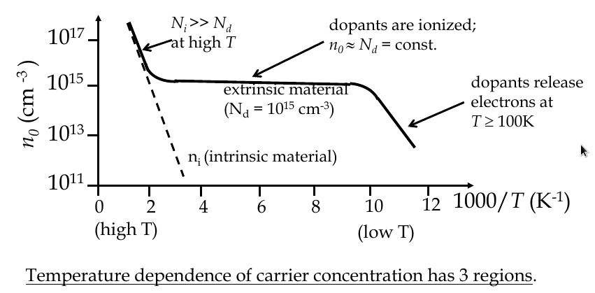
Temperature dependence of carrier concentration

$$ n_i (T) = 2{\frac{2\pi kT}{h^2}}^{\frac{3}{2}}{m_n^* m_p^*}^{\frac{3}{4}}e^{\frac{-E_G}{2kT}} $$

Compensation doping

• semiconductor could have both acceptors and donors in it: this is compensation doping
• the concentrations of electrons, holes, donors and acceptors can be obtained from space charge neutrality law
  • the material must remain electrical neutral overall
• p ₀ + N _d ⁺ = n ₀ + N _a ^-
• a material doped equally with donors and acceptors becomes “intrinsic” again

Diffusion Current

• diffusion: net motion of carriers from regions of high carrier concentration to low carrier concentration if there is non-uniformity (gradient) of carrier concentration

need more

Direction and indirect bandgap semiconductors

• dielectrics and semi-conductors behave essentially the same way - the only difference is the bandgap width
• photons with energy exceeding E _g are absorbed by giving their energy to electron-hole pairs
  • may or may not reemit the light during recombination depending on whether the gap is direct or indirect
• direct bandgap semiconductors: electron drops from bottom of CB to top of VB, excess energy emitted as a photon
  • also known as radiative recombination
• indirect bandgap semiconductors: recombination occurs in two stages via recombination centres (usually defects) in the bandgap:
  • electron falls from bottom of CB to the defect level, then down to the top of VB
  • electron energy is therefore lost in two portions by the emission of phonons (lattice vibrations)
  • this process is also known as non-radiative recombination

Photoconductivity

• increase of conductivity under illumination
  $$ \Delta \sigma = \sigma_photo - \sigma_dark = \frac{e\eta I\lamda \tau (\mu_e + \mu_h)}{hcD}
• η is quantum efficiency, and τ is average excess carrier lifetime

Energy-band diagrams and MOSFET

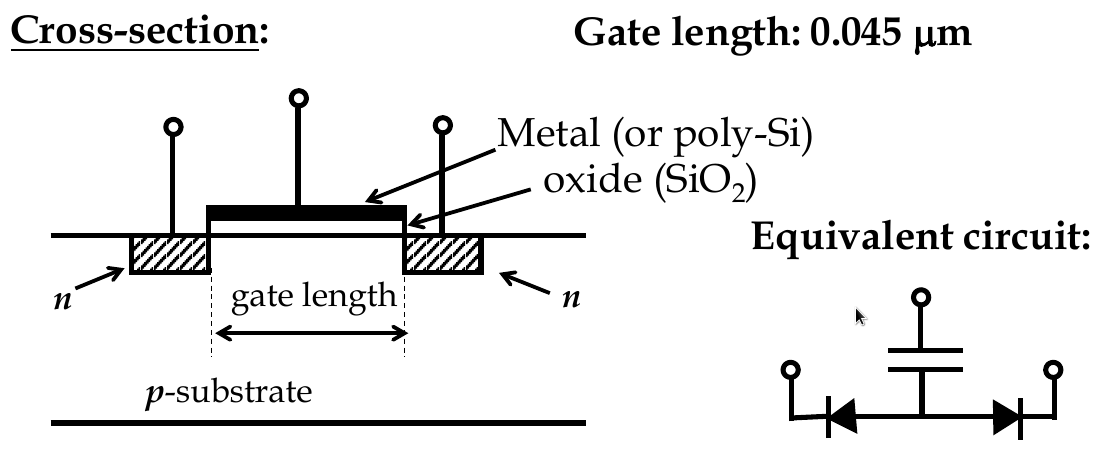
• no current from source to drain b/c diodes
• channel is conductive because gate electrode is used
• there is an insulator between metal and semiconductor, electric field builds across oxide layer if V is applied
  • similar to parallel plate capacitor

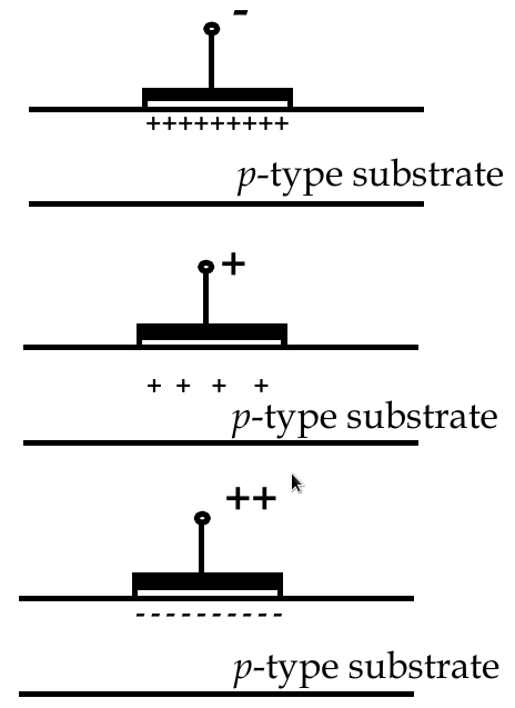
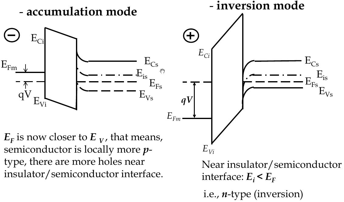
MOSFET Operation Modes

• accumulation mode
  • negative voltage at the gate increases number of holes at interface
• depletion mode
  • small positive voltage repels holes
• inversion mode
  • large positive voltage attracts electrons to the interface, making it locally n-type

MOSFET Band Diagrams

• to build energy band diagrams:
  1. choose zero points on co-ordinates (for energy axis, 0 is vacuum level)
  2. in equilibrium, E _F = const everywhere on band diagram xo
     

Metals

Critical issues with metallization

• more devices per unit area - more metal interconnection lines
• issues:
  • longer interconnects
  • higher capacitance per unit area
  • increasing heat (more devices per chip and higher frequency => increased heat production)
• interconnects: resistance is R =ρl/A, resistance increases as width/length decrease
• capacitance: metal lines end at MOSFET gate, forming RC line - potential source of slowing down the circuit speed
• heat production: at junctions between metal layers, metal is thin => resistance higher, higher heat production

Metallic bonding

• metal atoms have 1 to 3 valence electrons and ionize easily
• electrons are shared between all atoms, so metal ions are surrounded by electrons
• electrostatic forces are equal in all directions
  • ions positions are fixed
  • electrons move around freely

Electrons in metals

• in a perfect metal crystal at T=0, there is no resistance due to the wave nature of electrons
• an electron moving at constant velocity behaves as a plane wave
  • after interactions with wave, ions become the “sources” of secondary wavelets
    $$ n\lambda = 2dsin\theta $$
• in case of small interatomic distance and low electron speed
  $$ \lambda > 2d \\ \frac{\lambda}{2d} = \frac{sin\theta}{n} > 1 $$
• only solution is at n=0, θ=0
  • transmission occurs in direction of travel, magnitude unchanged
• source of resistivity is either the temperature or non-crystallinity of a metal

Temperature dependence of resistivity

• At T>0K, atoms move away from ideal lattice position b/c vibrations
  • electrons become scattered
• for atoms in a gas:
  • mean free path: average electron path length is defined
  • mean free time: time between collisions

In the Presence of an Electric Field

• when a potential difference is applied across metal, electrons drift towards larger positive potential
• current density:
  $$ J = nqv^d$$

Drift Velocity

• in electric field, electrons experience acceleration
• electron collisions with lattice ions causes velocity loss
• net acceleration of electrons between collisions
  $$ \frac{dv_d}{dt)_ACC = frac{-q\epsilon}{m} $$
• velocity loss at each collision:
  $$ \frac{dv_d}{dt}_LOSS = \frac{-v_d}{\tau} $$
  $$ \frac{dv_d}{dt}_TOTAL = \frac{v_d}{\tau} + frac{-q\epsilon}{m} = 0 $$
• mobility: μ = qτ/m

Phonons

• due to bonding, atom motions are connected (behave like a wave)
• types of wave motion:
  
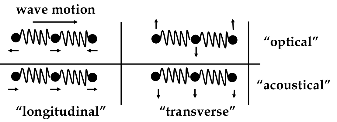
• these waves act like phonons
• can model interaction between lattice and electron wave as interaction between electron and phonon

Structural dependence of resistivity

• structural disorder gives rise to resistivity
• list of imperfections in a chip includes:
  • impurity atoms
  • dislocations
  • grain boundaries

Superconductivity

• for many elemental metals and alloys, the resistivity falls to an immeasurably small value at some point before the critical temperature (T _C )

The Meissner Effect

• when superconducting material at temperature above T _C is placed in a magnetic field and then cooled down, all magnetic field lines are ejected from the material at T=T _C

Optical Properties

Light wave propagation, Refraction Index

• the velocity of the wavefront of light depends on the material in which it is travelling (because waves, yo)
  • in dielectric non-magnetic material, electric field part of the wave interacts with electrons etc, polarizes atoms and molecules at the frequency of the wave
  • since wave propagation is coupled with dipole formation, polarization slows down propagation
• rate of propagation is characterized by dielectric permittivity and magnetic permeability
  $$ v = \frac{1}{\epsilon_r \epsilon_0 \nu_r \nu_0} $$

Refraction Index

• refraction: the bending of light as it passes from one material to another (due to the change in velocity)
• refraction index is n = c/v , v = speed of light in material
  • is a consequence of electric polarization
• when a light wave passes through a material, energy is lost to the electrons of the material
  • energy transferred comes from the velocity change
• since polarization is frequency dependent, refractive index also depends on the wavelength of light

Dispersion

• dispersion: a general name give to effects that vary with wavelength
  • wavelength dependence of the refractive index is the dispersion of the refraction index
    $$ n^2 = 1 + \frac{A_1 \lambda^2}{\lambda^2 - \lambda_1^2} + \frac{A_2 \lambda^2}{\lambda^2 - \lambda_2^2} + ... } $$
• A _n and λ _n are the Sellmeier coefficients
• since white light is a collection of multiple wavelengths, its velocity is a group velocity , and has a group index

Snell’s Law, Total Internal Refraction

• angles of incidence and refraction are related by Snell’s Law
  $$ \frac{sin\theta_1}{sin\theta_2} = \frac{v_1}{v_2} = \frac{n_2}{n_1} $$
• in the case n ₂ < n ₁ , refraction angle θ ₂ exceeds 90º, the light does not exit material 1 but is totally internally reflected
• respective incidence angle is called critical angle θ _c
  $$ sin\theta_c = \frac{n_2}{n_1} $$

Optical Fibers

• got that total internal reflection going on
• fiber optic tech has super fast speed of data transmission
• HELP

Photon interaction with materials. Absorption, Reflection, Transmission, Refraction

-from conservation of light, I ₀ = I _T + I _A + I _R ,
- I ₀ is the intensity of incident light, I _T , I _A , I _R are intensity of transmitted, absorbed, and reflected light
- three types of light-material interactions:
- transmission
- absorption
- reflection
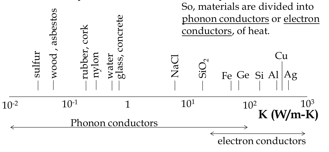
- materials divided into:
- transparent (little absorption and reflection)
- translucent (light scattered within material)
- opaque (relatively little transmission)
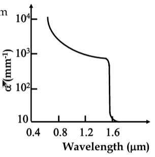
- if material not perfectly transparent, light intensity decreases exponentially with distance
- if the light intensity drop in δx is δI δI = -α δx I
- α = absorption co-efficient (m ^-1 )

Bouger-Lambert-Beer’s Law

$$ ax = -ln(frac{I}{I_0}) $$
- light could be absorbed by the nuclei (all materials) or by the electrons (metals and narrow E _g semiconductors)

Atomic Absorption

• type of absorption strongly depends on the type of material that absorbs
• ionically bonded solids show high absorption because oppositely charged ions move in opposite directions creating more interactions
• phonons exist in bands but only one of the phonon energies is excited by the radiation, so there is only one absorption frequency
• transmission spectrum shows just one dark and is called line spectrum
• absorption spectrum is dominated by the absorption due to the molecules themselves
• air pollution monitoring: can fitting known spectra of various gases to the measured atmospheric spectra over the same frequency range

Absorption in Metals

• in metals, photons are absorbed by electrons
  • almost any frequency of light is absorbed
• practically all light absorbed within about 100nm of metal surface; thinner metal films will partially transmit light
• excited electrons in the surface layers of metal - recombine again, emitting the light
  • metals are both opaque and reflective
• reflection can be explained in terms of electrostatics
  • EM field forces the free electrons to move, moving charge is source of EM waves. Therefore, wave is reflected
• band structure of metals not as simple as we assumed - there can be absorption below E _F
• metals are more transparent to very high energy radiation, where the inertia of electrons is the limiting factor

Absorption in Non-Metals

• dielectrics and semiconductors behave essentially the same way - only difference is the bandgap width
• photons with energy exceeding E _g are absorbed by giving their energy to electron-hole pairs
  • may or may not re-emit the light during the recombination, depending on whether the gap is direct or indirect
  • direct bandgap: excess energy emitted as a photon
  • indirect bandgap: energy is lost in two portions by the emission of phonon (lattice vibration)
    

Reflection

• occurs at the interface between two materials and is therefore related to refraction index
• reflectivity is the ratio of incident and reflected light intensities
  • R = I _R /I ₀
• assuming light is incident normally to the interface
  $$ R = \frac{n_2 - n_1}{n_2 + n_1}^2 $$

Transmission

• reflection and absorption are wavelength dependent
• transmission - a “leftover” after reflection and absorption
• to get transmission spectrum, just subtract reflection and absorption spectra from the incident light spectrum
  $$ I_T = I_0 - I_A - I_R $$
• small differences in composition may lead to large differences in appearance

Colours

• Al ₂ O ₃ (sapphire) is colourless - adding 0.5-2.0% of Cr ₂ O ₃ turns the material red - ruby!
• Cr atoms substitute Al in the crystalline lattice and introduce impurity levels in sapphire bandgap
  • these levels give strong absorption at 400nm (violet) and 600nm (orange), leaving only red light to go through
• similar technique is used to colour glasses by adding impurities while in the molten state

Emission. Luminescene and Fluroscence

Emission in Non-Metals - Luminescence

• luminescence: general term which describes the re-emission of previously absorbed radiative energy
  • common types: photo-, electro-, cathodoluminescence
  • depends on source of incident radiation: light,(fluorescent light) electric field (LED), or electrons (CRT)
  • also chemoluminescence due to chemical reactions (which makes glow sticks)
• luminescence is further divided into phosphorescence and fluorescence
• fluroescence: electron transitions that require no change of spin
• phosphorescence: electron transitions that require a change of spin
• hence, fluroescence is faster!

Luminescence

• if the energy levels are actually a range of energies, after electron excitation we observe a series of transitions accompanied by phonon emission, and then fluorescent transition
• since part of electron energy is released as phonons, then the light emitted by fluorescence is of longer wavelength than incident light

Lasers

• LASER: Light Amplification by the Stimulated Emission of Radiation
• before, we considered spontaneous light emission, which happened due to randomly occurring effects
• stimulated emission refers to electron transmissions that are stimulated by the presence of other potons
• an incident photon with E >= E _g is equally likely to cause stimulated emission of another photon as be absorbed
  • emitted photon has the same energy and phase as the incident photon (i.e. they are coherent)
• normally we have less electrons in the excited state than ground state
  • if we somehow get more electrons in the excited state than ground state, than we get stimulated emission -> much more photons in the output than in the input -> we get amplification
• population inversion: when we have more electrons in the excited state than in the ground state
• since random spontaneous emission gives incoherent output, it should be minimized in LASERs
  • done by using transmissions from which spontaneous emission is less likely; transmission from metastable states

• common material for solid state lasers is ruby, sapphire with Cr impurities
• to make laser, we have to achieve
  • population inversion
  • enough photons to stimulate emission
• first condition is met by filling the metastable states with electrons using a zenon flash lamp (in ruby laser) or by electron injection (in semiconductor laser)
• second condition is achieved by making laser in the rod shape. By mirroring the ends of the rod, we let photons travel back and forth along the rod
  • in order to keep the coherent emission, we must ensure that the light completes the round trip between the mirrors and returns in phase with itself
• in order to produce coherent output, the distance between the rod ends must obey the relationship:
  nλ= 2L

• in semiconductor lasers, thin films of direct semiconductors are epitaxially deposited on top of each other
  • central layer is degenerately doped (the doping is so heavy that E _F < E _V and there are lots of empty electron states in the valence band)
  • under bias, electrons are injected from n-layer into central later and get trapped there
  • thus, population inversion in central layer

Dielectric Materials

• dielectrics increase the capacitance between parallel plates
  $$ C + \frac{\epsilon_o \epsilon_r A}{d}
• increased capacitance allows more charge storage
  • Q = CV
• why do we care about studying dielectric materials?
  • electron devices become smaller! A is always decreasing as the devices shrink; d cannot decrease indefinitely as bellow 5-10nm, tunnelling occurs. Therefore you get less charged stored as devices shrink.
  • but you cannot increase V too much as breakdown will occur. So the only way to increase C is to the increase the relative permittivity, which depends on the dielectric
• types of dielectric materials:
  • MOSFETs: charge has to be accumulated at the semiconductor/gate dielectric interface
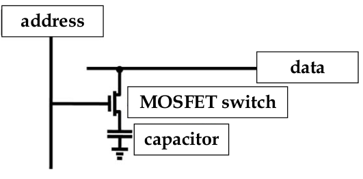
  • DRAM: charge is injected and retained in a capacitor with a MOSFET switch
  • CCD cameras: charged generated by photons is retained in the capactiros and read out by charge transfer between them
  • LCD: each pixel is a capacitor; charge stored generates E-field across liquid crystal layer and causes LC molecules to rotate

Surface Charge and Surface Electricity

• dielectrics are insulators; do no conduct electric current at room temp
• electric charge deposited on the dielectric surface cannot move and stays on the surface (e.g. being attached to surface defects)
• dielectrics are therefore efficient in storing electrostatic charge!

Surface Charging

• electron interactions at surfaces are complex and still poorly understood
• all materials have “surface states” caused by the incomplete bonds
  • strongly affect the behaviour of many electronic devices
• all ICs are covered with protective layer (‘passivation’) to prevent contamination by water vapour, etc.
• many materials that bond covalently or ionically charge positively when rubbed
  • friction removes unbonded electrons
• however, polymer-based materials tend to charge negatively:
  • consider a material like paraffin. The side-arms of molecular structure tend to attract water. Friction removes the H+ ions, leaving the OH- behind

Coulomb’s Law

• summary of electrostatics:
  • like charges repel, opposites attract
  • the force between charges:
    • inversely proportional to distance ²
    • dependent on surrounding medium
    • acts along a line joining charges
    • proportional to each charge

• Coulomb’s Law:
  $$ F = \frac{q_1 q_2}{4\pi \epsilon r^2} u $$

• in dielectrics, ideally no electrons available in the conduction band

• in reality, some electrons are present caused by random phenomenon (e.g. UV rays, cosmic rays)
  • will be a small leakage current

Capacitance Effects: Fringing Fields

• simple expression for capacitance has ignored several factors - most important being Edge effects
• electric field at the edges of a capacitor is non-uniform
• edge effects are important also when considering the RC time constants of the IC interconnects (higher RC values limit the speed of the ICs)
• fringing fields increase the effective area of the capacitor, leading to significant error
• in ICs, also have to consider capacitive coupling between metals in different layers causing crosstalk

Polarization and Relative Permittivity

What Happens: Dielectric Between Plates of a Capacitor

• more general definition of electric field: E _x = -dV/dx = -∇V
• when a dielectric is inserted into parallel plate capacitor, additional charge is being stored on the plates
  • relative permittivity increases as a result
• increase in the stored charge is due to polarization of the dielectric in the electric field
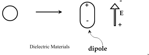
  • atoms and molecules become polarized when they are subjected to an electric field, and form electric dipoles

• polarization occurs when voltage is applied to capacitor - first electron’s worth of charged is induced on the plates
  • the charge causes the dielectric to polarize, and therefore does not contribute to building up the potential difference across the capacitor
  • this same thing happens to the next electron’s worth of charge -> until all atoms in the dielectric are polarized
  • only then due charge induced on capacitor start to contribute to build up the potential difference across the capacitor
• therefore more charge has to flow in before capacitor charged up to the supply voltage
  • charge storage capacity has increased
  • dielectric has increased its capacitance

Polarization

• in the presence of electric field, centres of each charge become slightly misplace and the particles become polarized - electric dipoles
• polarization is equal to the bound charge per unit area of the dielectric surface; measured in Coulombs/m ²
• dipole moment: the (absolute) charge on each of the two dipoles separated by their distance
  • μ= Qd
• consider P bound charges per unit area on opposite sides of a cube with side l, A = l ²
  • oppositely direct dipoles inside the cube cancel out each other; the only uncompensated charge is next to the surfaces of the cube
  • total dipole moment is therefore: μ= P A l
  • P is electric dipole moment per unit volume
• INSERT MORE HERE 23-24

Polarization Mechanisms

• dipole moment also depends on the electric field within the material
  • remember that zero field gives no polarization, so μ must be field dependent
• μ= αE _int
  • α = polarizability of the material
  • the average dipole moment per unit of internal field
• Clausius Equation:
  • P = (ε _r - 1)ε _o E = N αE _int
• several mechanisms that contribute to α: α = α _e + α _a + α _d + α _i
  • α _e : electrical polarizability
  • α _a , α _d : molecular polarizability
  • α _i : interfacial polarizability

Electrical Polarizability

• also called optical polarizability because the polarization can keep up with even optical frequencies
• with no electric field, electron clouds are symmetric around the nucleus
  • when field is applied, electron cloud is distorted
• the centers of the negative and positive charges are now offset, leading to an electric dipole μ _e = α _e E _int

Molecular Polarizability

• arises when the molecules of the material naturally forms dipoles (e.g. H ₂ O)
• two things can happen when an electric field is applied:
  • atomic polarizability α _a
  • orientational polarizability α _d
• no α _d in ionically bonded solids because strong bonding forces prevent wholesale re-alignment of molecules
  • however, small change in “centre of mass” of the bonds so a small α _a can be present

Interfacial Polarizability

• accounts for the presence of lattice imperfections, ionized contaminants, a few electrons etc.
• in an electric field, some or all of these can move through the material until they come to an interface

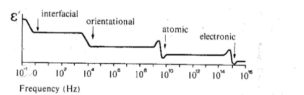
Frequency Dependence of Polarization

• how do we distinguish the effect from different types of polarization?
• if you put a dipole in an alternating field, the dipole will attempt to follow the oscillating field
  • but the dipole has inertia, so it takes a finite time to respond to field
• if we oscillate the field fast enough, the dipole will eventually cease to respond fast enough
• relaxation frequency: the frequency at which the dipoles cannot move at all before the field reverses direction (hence the polarization “goes away”)
  • relaxation occurs at different frequencies for different mechanisms of polarization
• relaxation frequency higher when switching smaller masses of material (less inertia)
• so if we plot the permittivity as a function of frequency, should find changes at each relaxation frequency
• electronic: only electrons must be moved, they’re very light so relaxation occurs at high frequencies
• atomic: relies on ions moving their positions so freq should be about the same as thermal oscillations of the atoms
• orientational: requires reorganization of groups of dipoles - freq lower than atomic
• interfacial: caused by charge that percolates slowly through entire thickness of material; very low freq

Classification of Dielectrics

• classify dielectrics into three categories:
  • non-polar materials: show variations of permittivity in the optical range of frequencies only
  • polar materials: display both atomic and electric polarizability
  • dipolar materials: display atomic, electric, and orientational polarizability

AC Permittivity and Dielectric Loss

• dielectrics may have different response time in case of AC voltage
• current leads the voltage when voltage applied to capacitor
• in a real capacitor, there will be a small leakage current through the dielectric, which will be in phase with V
• thus, real capacitor consists of a capacitive component connected in parallel with a resistive component

• since the impedance now consists of real and imaginary components of 0 ^o and 90 ^o phase, total phase difference is slightly less than 90 ^o , by δ ^o
• δ is the loss angle
• mathematically, this is accounted for by defining the permittivity to be a complex number:
  • ε _r = ε ^’ - jε ^’‘
  • loss angle is therefore tanδ = ε ^’‘ /ε ^’
• since power dissipated in the capacitor is proportional to the value of ε ^’‘ , dielectrics want as small a δ as possible
• capacitive component of the capacitance has the same frequency dependence as the polarizability
  • resistive component of the capacitance has several maxima at the frequencies at which capacitive components of the capacitance cease to respond
  • these frequencies (relaxation peaks) should be avoided due to power dissipation

Gauss’ Law and Boundary Conditions

• what if we have non-uniform dielectric between the plates of the capacitor?
• electric flux density, D, in the material is given by: D = εE
• from Coulomb’s law, we get:
  $$ D = \frac{q}{4\pi r^2} a $$
• this means D is independent of ε for fixed q
• the total flux crossing the sphere area is given by D*Area
• this leads to:
  $$ Flux = 4\pi r^2 \frac{q}{4\pi r^2} = q $$
• total flux out of the surface is equal to the enclosed charge; the generalization of this to all closed surfaces is Gauss’ Law

Dielectric Breakdown

• we cannot apply an infinitely large voltage across our capacitor without it breaking down
• dielectric breakdown usually evidenced by a sudden increase in current to a very large value
• breakdown voltage (V _BD ): voltage that causes dielectric breakdown
• dielectric strength (E _BR ): maximum electric field that can be applied to a dielectric without a breakdown
• in real insulators, breakdown voltage can be hard to predict since it depends on surface and ambient conditions

Breakdown Mechanisms

• avalanche breakdown: occurs if the electric field across the insulator is high enough
  • the few electrons present can achieve enough energy to ionize other atoms (impact ionization)
  • secondary electrons are also accelerated, causing further ionization and avalanche develops
• thermal breakdown: occurs if the leakage current (loss angle) is large enough to cause significant heating -> more leakage -> more heating
• discharge breakdown: occurs is small gas bubbles are present in the material

Capacitors and Memories

• main applications of dielectrics in electronics: capacitors and memory cells
• capacitors: can be made as discrete elements or be integrated with other elements on the same wafer
  • discrete caps made from alternating layers of metal and dielectric, wrapped up in a package
  • dielectric material is chosen to get the right range of values with the minimum loss angle

RAM

• same problem of fitting capacitor into a small space occurs with RAM cells
• in RAM, SiO ₂ is used as the dielectric
• data is stored as the charge in a capacitor cell with a MOSFET as a switch

• as the devices shrink, the challenge is how to maximize the charge storage and minimize the cell area
  

• reducing cell area is important for increased storage densities

  • chip manufacturers make the capacitors 3D, which requires complex fabbing and may be more susceptible to faults
• could increase charge storage capacity by using another material but manufacturers are slow to change their fabbing process

Piezoelectric Materials

• piezeoelectric materials: a mechanical stress (tension or compression force/area) causes a dielectric polarization or an applied electric field will cause a mechanical strain
• used for electromechanical sensors and actuators
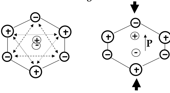
• mechanism of piezoelectricity involves an asymmetry in the arrangement of positive and negative ions in the material
• have a hexagonal unit cell
  • with no pressure applied, the centers of positive and negative charges concide
  • when mechanical pressure is applied in the vertical direction, the centers split - a dipole forms

• symmetric material would not change its dipole moment when stressed
• pressure applied in the horizontal direction does not induce polarization - piezoresistivity is anizotropic
• polarization, P, is related to mechanical stress, T
• electric stress, E, is related to the mechanical strain, S
  $$ d = (\frac { \partial P}{\partial T})_E = (\frac { \partial S}{\partial E})_T = "polarization coefficient" $$
• quartz is historically the first piezoelectric material
  • quartz crystal is cut into a disc and electrodes are plated onto opposite sides
  • now, the disc has a mechanical resonant frequency precisely determined by its size
  • we can excite mechanical oscillations by applying an AC voltage
  • the resonant frequency of that voltage is therefore the same as that of the mechanical oscillation

Thermal Properties of Materials

Heat Issues in ICs

• electrons release their energy to vibrating atoms upon collisions, causing heating
• if generate heat is not removed, temperature increases
• consequences:
  • carrier mobility may change
  • carrier concentration may change
  • dielectrics may leak more or even break down
• heat generation in IC due to electric power:
  • P = IV = JAV = V ² /R = I ² R
• total generated heat increases with:
  • more devices or interconnection lines per unit area (higher J)
  • higher operating voltage
  • higher operating frequency

Mechansms of Heat Generation and Loss

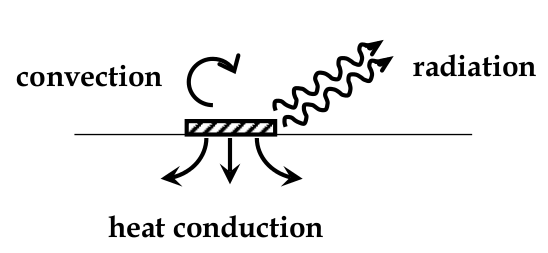
• heat loss mechanisms in IC:
  • heat conduction
  • heat radiation
  • convection
• heat conduction: flow of heat through a solid, analogous to electronic transport but with:
  • driving force being ΔT instead of ΔV
  • constant of proportionality is thermal conductivity instead of electrical conductivity
• heat radiation : loss of energy by the emission of EM radiation in the IR wavelengths
• heat convection: transfer of heat away from a hot object because the gas next to it heats up and becomes less dense and then rises
  • currents of gas flow

Overview of Heat

• heat (Q) flows from hotter objects to cooler
• First Law of Thermodynamics: ΔE = W + Q

Heat capacity

• heat capacity (C): ability to absorb heat from the external surroundings; amount of energy needed to heat particular material
  • dQ = CdT
• depends on conditions measured under (volume and pressure)
  • C _P ^’ : under constant pressure
  • C _V ^’ : under constant volume
    $$ C_V^\prime = C_P^\prime - \frac{\alpha TV}{K} $$
• specific heat capacity: heat capacity by unit mass
  $$ c_p = \frac{C_P^\prime}{m} $$
  $$ c_v = \frac{C_V^\prime}{m} $$
• molar heat capacity: heat capacity per moles of atom
  $$ C_V = c_vM = \frac{C_V^\prime} {n} $$

Dulong-Petit Law

• C _p = C _v = 25 J*mol ^-1 K ^-1
• Dulong-Petit Law: heat capacity of metals saturates at 25 J*mol ^-1 K ^-1
• heat capacity and thermal conductivity can be calculated by:
  • classical theory based on thermodynamics
  • quantum mechanics based on interaction

Thermal Conductivity

• thermal conductivity (K): proportionality coefficient between heat flow density and temperature gradient
  • ability to conduct heat
• Fourier’s Law:
  $$ J_Q = -K\frac{dT}{dx} $$
• slightly temperature dependent, usually decreases as temperature increases

Classical treatment of heat capacity

• treat electrons in a metal as a gas
• ideal gas law: PV = nRT
  • will use in calculation of kinetic energy of gas molecules (or electrons in a metal)
• in a small volume of gas, about 1/3 on average will move in x-direction - 1/6 will move in +x direction
• number of particles per unit time that hit the end of the volume per unit area will be:
  $$ Z = \frac{1}{6}n_v v $$
  • where v= velocity, n _v = particles per unit volume
• momentum transferred per unit area is:
  $$ p^* = Z2mv = \frac{1}{6}n_v mvm = \frac{1}{3}\frac{N}{V}mv^2 $$
• we find that the average kinetic energy of a gas molecule:
  $$ E_kin = \frac{3}{2} kT $$
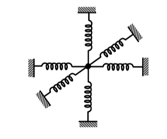
• atoms vibrate about their ideal lattice positions due to their thermal energy
  • such an atom can be thought of as being like a sphere supported by springs
• the atom acts like a simple harmonic oscillator which “stores” an amount of thermal energy
  • E = kT
• in a three-dimensional solid, oscillator has energy E = 3kT; energy per atom
• total internal energy per mole is therefore: E = 3N _o kT

$$ C_V = \frac{\partial E}{\partial T} = 3kN_o $$
- classical treatment works well at high temperatures
- implies that heat capacity is constant and independent of temperature
- however, heat capacity is dependent on temperature
- Debye Temperature (θ _D ) : temperature at which C _V has reached 96% of its final value

Quantum Theory of Heat Capacity

• key assumption: the energies of the “atomic oscillators” are quantized
  • such quantized lattice oscillations are called phonons
• number of phonons increase with temperature
• energy of each phonon is constant (electrons - number is constant but energy changes)
• Bose-Einstein Distribution : the average number of phonons at any temperature was found to obey a distribution
• turns out, electrons play a small part in the heat capacity; only a small fraction of the total number of electrons can gain thermal energy
• 1% of C _V is contributed by electrons at room temperature

Quantum treatment of thermal conductivity

• what is the mechanism of heat transfer?
• in a solid, only two things can move:
  • electrons
  • phonons
• depending on the material, either one or the other tends to dominate
• good electrical conductors tends also to be good thermal conductor
• Wiedemann-Franz Law: relationship between electrical and thermal conductivities (for metals), suggesting that electrons can carry thermal energy as well as electrical
• because of electrical neutrality, equal number of electrons move from hot -> cold and from cold -> hot
• but their thermal energies are different and so the heat transported is proportional to the difference between electrical and thermal energies
• in electrical insulators, there are few free electrons so the heat must be conducted in some other way - phonons (lattice vibrations)
• the major difference between conduction by electrons and by phonons:
  • electrons: number constant but energy varied
  • phonons: number is variable (more phonons at hot end) but energy is quantized

Classical theory of Thermal Conductivity

• let us consider a bar of material with a thermal gradient dT\dx
• we calculate the flow of energy through a volume due to the temperature gradient and use this to calculate the number of “hot” electrons
• an equal number of “cold” electrons must flow the opposite way, so we can solve for K

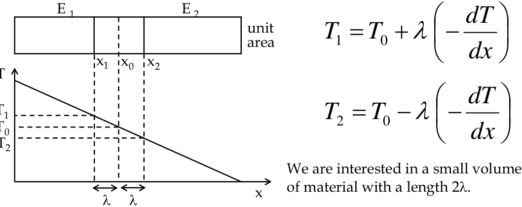
- λ is the mean free path between collisions with the lattice
- the idea is that an electron must have undergone a collision in this space and hence will have the energy/temperature of this location

Wiedemann-Franz Law

$$ \frac{K}{\sigma T} = \frac{\pi ^{2 k} 2}{3q^2} = L $$
- L = Lorentz number
- works quite well for metals, but not for “phonon materials”

Thermal resistance

• just as we can relate electrical conductivity to electrical resistance, we can obtain a thermal resistance
• for the temperature of the device on the chip:
  • T _j = T _a + θ _ja P
  • T _j junction temperature
  • T _a ambient temperature
  • P dissipated power
  • θ _ja junction-to-air thermal resistance
• θ _ja can be composed of several resistances in series
  • θ _ja = θ _D + θ _j1 + θ _P + θ _j2
  • θ _D chip
  • θ _j1 chip-to-package
  • θ _P package
  • θ _j2 package to air
• would like to minimize θ _ja in order to get a smaller drop in temperature per unit power
• recall we can lose heat due to radiation, conduction, and convection
  • all of these depend on surface area, so we can improve heat dissipation by using a high sink of high thermal conductivity

Magnetic Properties

Basic Concepts

Faraday’s Experiment

• in non-uniform magnetic field, diamagnetic materials are ejected while others are attracted to different degree

• A force: F = VH(dH/dx)

  • where H = magnetic field strength
  • V = sample volume

• two constants are used to characterize magnetic properties:

  • susceptibility: χ, “responsiveness” of material
  • permeability: μ = (1 + χ)μ ₀
  • μ ₀ = permeability of free space
• magnetic field strength, H is related to magnetic field density, B
• outside the material: B ₀ = μ ₀ H
• inside the material: B = μ ₀ (H + M)
  • where M, magnetization of material is proportional to H: M = χH

Para- and Dia-magnetics

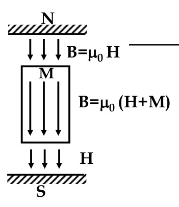
Paramagnetic and Ferromagnetics:
$$ B = \nu H = \nu_0 (H + M) $$

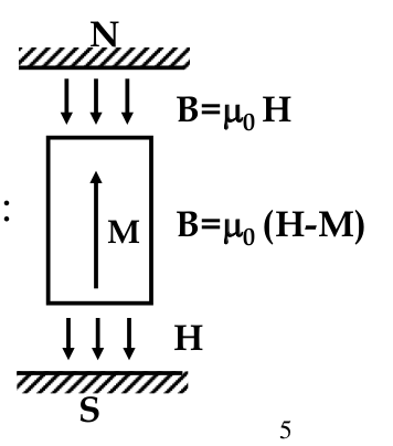
Diamagnetics:
- M opposes H
$$ B = \nu H = \nu_0 (H - M) $$

Magnetic Moments

• magnetic materials always act as dipoles (even as a small piece of magnetic material, carries double magnetic charge - N and S poles)
• therefore, possible to define a magnetic dipole moment
• each atom of magnetic material acts as a magnetic dipole
  • electric orbits acts like a coil generating magnetic field.
  • the material can be considered as an assembly of blocks - current loops
• the magnitude of magnetic dipole μ _m = Ai
  • A = area of current loop
  • i = value of the current in the loop
• in macroscopic body, net current in interior blocks is 0 because neighbouring currents cancel each other
  • on the surface, there is non-zero net current which equals iAn, where n is the number of blocks
• every atoms except noble gases should demonstrate magnetic properties (inequal number of +- m _l and +- m _s )
  • this is valid for gases only
• all magnetic compound materials include at least one transition element
  • these elements have an inner incomplete electron shell
  • as we learned, when atoms bond they electrons fill their * outer electron shell
  • only materials with incomplete inner shells after bonding show magnetic properties

Size of Atomic Magnetic Moment

• when atomic sub-shells are being filled, the m _l are first filled with electrons have m _s = +1/2 and only then electrons having m _s = -1/2 start to occupy their states
  • the consequence of this is that electrons with two different functions and the same spin have a lower energy then electrons with different wave functions and different spins

Bohr Magneton

• β = qh/4πm - fundamental unit of magnetic moment

Alignment of Magnetic Moments in a Solid

• rules for magnetic solids:
  • closed shells give no magnetic moment
  • this is no μ _orb for 3d shells
• third effect is the interaction between the electron spins of adjacent atoms
  • this interaction can vary in strength. When it is strongest, it caries magnetic moments of adjacent atoms to either be parallel or anti-parallel to each other

Paramagnetics

• spin interactions are negligible compared to thermal agitation of the atomic magnetic moments
• directions of magnetic moments in atoms are randomly oriented
  • an external magnetic field can induce some degree of alignment but it disappears when field is removed

Ferro-, Antiferro- and Ferrimagnetism

Ferromagnetics

• strong spin interactions cause the atomic magnetic moments to align parallel to each other
• in these metals, 3d electrons from the incomplete shells can move around the materials
  • the ability of electrons to move reduces the interaction ebtween the electrons and hence the magnetic moments are also reduced

Antiferromagnetics

• strong spin interactions lead to these atomic magnetic moments to be anti-parallel to each other in adjacent atoms
• in the whole material, the number of atoms with anti-parallel magnetic moments are equal
  • net magnetic moment in the material is zero

Ferrimagnetics

• the moments for adjacent atoms are in opposite directions HOWEVER the moments have different magnitudes, thus giving us a non-zero net magnetic moment
• this feature stems from the nature of these materials: they are all compounds
• ferrimagnetics are electrical insulators, unlike all useful ferromagnets
• ferrimagnetics can be used for high-frequency applications to avoid high eddy currents and resultant losses
• ferrimagnetic compounds are called ferrites

Diamagnetics

• in diamagnetics, intrinsic magnetic field is opposite to external field therefore it is expelled from the field
• all materials are diamagnetic, but the effect is weak and only shows up when none of the other effects are present
• diamagnetism arises due to Lenz’ Law: “when a magnetic is moved towards a loop of wire, it induces a current in the loop which in turn generates a magnetic field to oppose the magnetic’s motion”

Curie Temperature

• beyond a certain temperature, a material ceases to be ferromagnetic at all, and M drops to 0
• at T = 0K, all atomic moments are perfectly aligned as we assume in our calculation. At T > 0K, thermal excitation of atoms reduces the degree of alignment and M drops
• the temperature at which M -> 0 is known as the Curie temperature

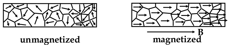
Domains and Hysteresis

• if all the atomic moments are lined up, this represents the maximum value of the moment - the condition known as saturation
• why are ferromagnetic elements not always permanent magnets?
  • materials are divided into sub-units known as domains
  • each domain is magnetized to saturation (inside domain, all moments are aligned)
  • however, direction of each domain can be randomly oriented

The B-H Curve

• since M relates B and H and M is not constant, what is the relationship between B and H in practice?
• H = external field, B = magentic flux density inside material

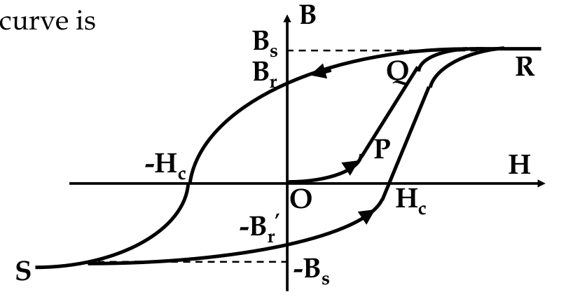
- as H increases, B follows the path O P Q R
- at R, B value saturates at B _s
- B _s corresponds to complete alignment of atomic moments
- if the applied field is now reduced after increasing to R, the path follows a different direction
- at H =0, B = B _r , known as remanence
- material now has a “permanent” magnetic flux density, becoming a permanent magnet
- to turn B to zero, apply a reverse field
- H _c = coercive field or coercivity
- if we further increase B in the reverse direction, get saturation at -B _s again
- hysteresis: the different behaviour of the B-H curve for different directions of H, and this curve is called the hysteresis loop

Hard and Soft Materials

• magnetic materials are divided into two broad groups based on their B-H curves: magnetically hard and magnetically soft materials
• this refers to how easy it is to magnetize or demagnetize them
• measure of magnetic hardness is the value of H _c
  • soft materials have a high permeability

Domains

• domain’s formation is caused by energy minimization reasons
• if all domains were aligned, then material would be magnetic and much of the field would be outside the material
  • but the field is a “storage” of potential energy called magnetostatic energy
  • the whole energy in the system could be reduced by forming more domains
• following this logic, the best result can be achieved if we have atomized domains
  • however, we have to consider the boundaries between domains, the domain walls
• domain wall: the boundary between the two domains where the magnetization changes from one direction to another and hence the atomic spins do too
  • not simply one atomic spacing wide
  • exchange forces between neighbouring atomic spins favour very little relative rotation
  • magnetic moments that are oriented away from the field direction possess excess potential energy call the anisotropy energy
  • in domain wall region, there is competition between exchange forces and the anisotropy energy minimization
• what happens when we apply external magnetic field to the ferromagnet?
  • domains aligned parallel to the field will expand at the expense of domains with other orientations
    • growth is called the motion of domain walls
• the stronger the magnetic field, the more non-parallel domains shrink. As their size is small enough, the magnetic moments in these domains can be rotated until the material is uniformly magnetic
  • in magnetically soft materials, domain size shrinkage and magnetic moments rotation occur simultaneously and at low field

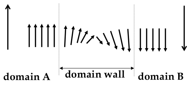
Domains in Polycrystals

• in polycrystalline materials, grain boundaries do not allow domain walls to expand
• after external field is applied, domain wall motion will result in crystal grains with single domains
  • in many grains, magnetic moments will be pointing at some angle to H
  • after we remove the field, some of these domains will return to previous conditions but some remain resulting in remanence B _r on the B-H curve
  • heat above T _c or strong reverse field -H use to reverse the effect

Magnetic Recording